Determination of Hydraulic Loss in Solidworks Flow  Simulation

In engineering practice the hydraulic loss of pressure head in any piping system is traditionally split into two components: the loss due to friction along straight pipe sections and the local loss due to local pipe features, such as bends, T-pipes, various cocks, valves, throttles, etc. Being determined, these losses are summed to form the total hydraulic loss. Generally, there are no problems in engineering practice to determine the friction loss in a piping system since relatively simple formulae based on theoretical and experimental investigations exist. The other matter is the local hydraulic loss (or so-called local drag). Here usually only experimental data are available, which are always restricted due to their nature, especially taking into account the wide variety of pipe shapes (not only existing, but also advanced) and devices, as well as the substantially complicated flow patterns in them.

Flow Simulation presents an alternative approach to the traditional problems associated with determining this kind of local drag, allowing you to predict computationally almost any local drag in a piping system within good accuracy. Click File, Open. In the Open dialog box, browse to the Valve.SLDPRT model located in the Tutorial 1 - Hydraulic Loss folder and click Open (or double-click the part). Alternatively, you can drag and drop the Valve.SLDPRT file to an empty area of the SolidWorks window.

Model Description

This is a ball valve. Turning the handle closes or opens the valve. The local hydraulic loss (or drag) produced by a ball valve installed in a piping system depends on the valve turning angle or on the minimum flow passage area governed by it. The latter depends also on a ball valve geometrical parameter, which is the ball-to-pipe diameter ratio governing the handle angle at which the valve becomes closed:

The standard engineering convention for determining local drag is by calculating the difference between the fluid dynamic heads measured upstream of the local pipe feature (ball valve in our case) and far downstream of it, where the flow has become uniform (undisturbed) again. In order to extract the pure local drag the hydraulic friction loss in the straight pipe of the same length must be subtracted from the measured dynamic head loss. In this example we will obtain pressure loss (local drag) in the ball valve whose handle is turned by an angle of 40o. The Valve analysis represents a typical Flow Simulation internal analysis.

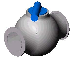
Internal flow analyses deal with flows inside pipes, tanks, HVAC systems, etc. The fluid enters a model at the inlets and exits the model through outlets. To perform an internal analysis all the model openings must be closed with lids, which are needed to specify inlet and outlet flow boundary conditions on them. In any case, the internal model space filled with a fluid must be fully closed. You simply create lids as additional extrusions covering the openings. In this example the lids are semi-transparent allowing a view into the valve

To ensure the model is fully closed click Flow Simulation, Tools, Check Geometry. Then click Check to calculate the fluid and solid volumes of the model. If the fluid volume is equal to zero, the model is not closed. Click Fluid Volume to see the volume that will be occupied by fluid in the analysis. Uncheck Fluid Volume. Close the Check Geometry dialog box.

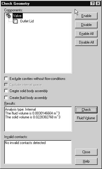
 The Check Geometry tool allows you to calculate the total fluid and solid volumes, check bodies for possible geometry problems (i.e. invalid contact) and visualize the fluid area and solid body as separate models. The first step is to create a new Flow Simulation project

1 Click Flow Simulation, Project, Wizard. The project wizard guides you through the definition of a new Flow Simulation project.
2 In the Project Configuration dialog box, click Use current. Each Flow Simulation project is associated with a SolidWorks configuration. You can attach the project either to the current SolidWorks configuration or create a new SolidWorks configuration based on the current one. Click Next.

3 In the Unit System dialog box you can select the desired system of units for both input and output (results). For this project use the International System SI by default. Click Next.

4 In the Analysis Type dialog box you can select either Internal or External type of the flow analysis. To disregard closed internal spaces not involved in the internal analysis, you select Exclude cavities without flow conditions. The Reference axis of the global coordinate system (X, Y or Z) is used for specifying data in a tabular or formula form in a cylindrical coordinate system based on this axis.

This dialog also allows you to specify advanced physical features you may want to take into account (heat conduction in solids, gravitational effects, time-dependent problems, surface-to-surface radiation, rotation). Specify Internal type and accept the other default settings.
Click Next.

Since we use water in this project, open the Liquids folder and double-click the Water item.  Engineering Database contains numerical physical information on a wide variety of gas, liquid and solid substances as well as radiative surfaces. You can also use the Engineering Database to specify a porous medium. The Engineering Database contains pre-defined unit systems. It also contains fan curves defining volume or mass flow rate versus static pressure difference for selected industrial fans. You can easily create your own substances, units, fan curves or specify a custom parameter you want to visualize.
Click Next.

6 Since we do not intend to calculate heat conduction in solids, in the Wall Conditions dialog box you can specify the thermal wall boundary conditions applied by default to all the model walls contacting with the fluid. For this project accept the default Adiabatic wall feature denoting that all the model walls are heat-insulated. In this project we will not consider rough walls. Click Next.

7 In the Initial Conditions dialog box specify initial values of the flow parameters. For steady internal problems, the specification of these values closer to the expected flow field will reduce the analysis convergence time.

For steady flow problems Flow Simulation iterates until the solution converges. For unsteady (transient, or time-dependent) problems Flow Simulation marches in time for a period you specify. For this project use the default values. Click Next

8 In the Results and Geometry Resolution dialog box you can control the analysis accuracy as well as the mesh settings and, through them, the required computer resources (CPU time and memory). For this project accept the default result resolution level 3.

Result Resolution governs the solution accuracy via mesh settings and conditions of finishing the calculation that can be interpreted as resolution of calculation results. The higher the Result Resolution, the finer the mesh and the stricter the convergence criteria. Naturally, higher Result Resolution requires more computer resources (CPU time and memory).

Geometry Resolution (specified through the minimum gap size and the minimum wall thickness) governs proper resolution of geometrical model features by the computational mesh. Naturally, finer Geometry Resolution requires more computer resources. Select the Manual specification of the minimum gap size check box and enter 0.04 m for the Minimum gap size.

Flow Simulation calculates the default minimum gap size and minimum wall thickness using information about the overall model dimensions, the computational domain, and faces on which you specify conditions and goals. However, this information may be insufficient to recognize relatively small gaps and thin model walls. This may cause inaccurate results. In these cases, the Minimum gap size and Minimum wall thickness must be specified manually. Click Finish.